4 Corpus Statistics
4.1 Word frequencies
4.1.1 Number of occurrences per article
The function stats_count provides statistics on the queried term(s). With the classic parameters, you can obtain the number of occurrences of this/these keyword(s) per article.
library(histtext)
df <- get_documents(search_documents("noble","ncbras"),"ncbras")
## [1] 1
## [1] 11
## [1] 21
## [1] 31
## [1] 41
## [1] 51
## [1] 61
## [1] 71
## [1] 81
## [1] 91
## [1] 101stats_count(df,"noble")##
## Attachement du package : 'plotly'## L'objet suivant est masqué depuis 'package:ggplot2':
##
## last_plot## L'objet suivant est masqué depuis 'package:stats':
##
## filter## L'objet suivant est masqué depuis 'package:graphics':
##
## layout4.1.2 Mean number of occurences over time
By adding the over_time=TRUE parameter, you can obtain the average values at which this keyword appears over the years
stats_count(df,"noble",over_time=TRUE)4.1.3 Percentage compared to other words over time
By adding the by_char=TRUE parameter, we can contrast the number of occurrences of the queried term with the overall number of tokens in the text per year.
stats_count(df,"noble",over_time=TRUE,by_char=TRUE)4.1.4 Plot or dataframe
For all statistical functions, it is possible to retrieve the statistics dataframe without generating the graph by setting to_plot=FALSE.
stats_count(df,"noble",over_time=TRUE,by_char=TRUE,to_plot=FALSE)## # A tibble: 52 × 4
## Date word_count search_term complete_count
## <dbl> <int> <chr> <int>
## 1 1858 3 noble 6062
## 2 1860 5 noble 22781
## 3 1864 12 noble 63253
## 4 1866 1 noble 2116
## 5 1867 1 noble 3308
## 6 1868 12 noble 77550
## 7 1869 2 noble 11299
## 8 1871 10 noble 28695
## 9 1874 2 noble 14553
## 10 1875 14 noble 36508
## # ℹ 42 more rows4.1.5 Interactivity
All visualizations are created using Plotly to make them interactive. However, it is possible to generate a non-interactive graph by deactivating ly=FALSE .
stats_count(df,"noble",over_time=TRUE,by_char=TRUE,ly=FALSE)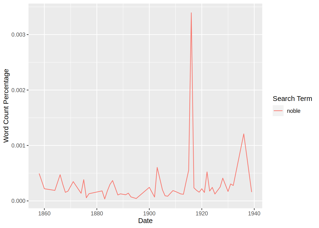
4.2 Characters count
The function count_character_bins counts the number of characters in the text and then groups them by “bins”, i.e. series of ranges of numerical value into which data are sorted in statistical analysis. It is possible to manually set the number of bins using the nb_bins argument, as shown below.
count_character_bins(df)count_character_bins(df,nb_bins=20)4.4 Document Term Matrix (DTM)
The classic_dtm function allows you to explore the semantic content of the text in more depth. To use this function, you need to have the following packages installed:
install.packages("stopwords")
install.packages("quanteda")
install.packages("quanteda.textstats")
4.4.1 Top words
The classic configuration allows you to see the top ‘n’ words present in the given texts. You can set the number of desired words manually using the top argument:
classic_dtm(df,top=20)## Package version: 3.3.1
## Unicode version: 13.0
## ICU version: 69.1## Parallel computing: 4 of 4 threads used.## See https://quanteda.io for tutorials and examples.